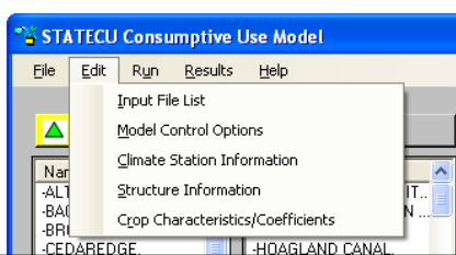
2.5 - Edit Menu
The Edit menu displays the major categories of StateCU input data that can be viewed and edited. All of the menu commands shown in Figure 19 are active for a simulation of crop consumptive use under a Structure Scenario, as described below. With a Climate Station Scenario, the Structure Information command under the Edit menu is not visible and the information shown under the Model Control Options and Climate Station Information windows is limited.
Figure 19 - Edit Menu (see also the full-size image)
Several input data files available under the Edit Menu allow the user to view and edit input data, including climate data, crop acreage, diversion records, and irrigation efficiencies. The ‘rules’ for editing input data through the GUI are similar for each data type, therefore the editing rules will be described in this section and referenced in the following sections when each data type is discussed individually.
The user has the ability to edit the input data through specific GUI windows, accessed through the main GUI Edit Menu. In all cases, input data can be edited for the existing time period provided in the scenario, however the user can not extend the time period of data. Input data through the GUI is provided in grid format, similar to an Excel spreadsheet. To edit an individual data value, select a cell, type-over the original data value and press ENTER, TAB or select a different cell to ‘commit’ the changed data value. Changed data values that are not ‘committed’ are not available to be saved when the save option is selected. Press ESC prior to committing a data value to retrieve the original data value.
There are commands available under each input data GUI window Edit menu to help the user edit the data, including Copy, Paste and Select All. The user can also click on a data cell with the RIGHT mouse button to access Copy, Paste and Adjust Values options. The Adjust Values options include Scale, in which the data value can be scaled up or down by a user-input value, or Add, in which the user inputs a value to be added (negative values are allowed) to the selected data value. Note that each data input type has allowable values, designed to provide minimal error checking and prevent the user from inputting unreasonable data. For example, diversion data must be between 0 and 100,000 and crop acreage data must be between 0 and 200,000. If the user provides a scale or addition factor that creates unreasonable data, the GUI will provide an error message indicating the scale or add operation was not successful and the allowable values for that specific data type.
Data can be copied and pasted into and out of the GUI window from an external spreadsheet or database application. Data can also be copied from one area of the GUI window to another area. Note that only allowable values can be pasted into the GUI window. Similar to the scale and add factor checking, minimum error checking will take place on the copied value(s) and the GUI will provide an error message indicating that the pasting operation was not successful and the allowable values for that specific data type. There are four possible configurations for pasting data into a GUI window; the GUI pastes each configuration in a similar fashion as Excel. The following list discusses the configurations and how the GUI handles each pasting operation:
- Copy one cell from the original source and paste one cell into the GUI window: The copied single data value will replace the GUI data value.
- Copy one cell from the original source and paste a range of cells into the GUI window: The copied single data value will replace all of the data values in the selected range in the GUI.
- Copy a range of cells from the original source and paste to one selected cell into the GUI window: The copied range of data values will replace the same number data values in the GUI, using the single cell selected as the upper left cell of the copied range. If the range to be pasted extends into read-only columns or rows (e.g. cells containing years, annual totals, etc.), then the pasted data will be truncated at that row and column. Note that if any of the copied data values are non-allowable, then none of the cells will be pasted.
- Copy a range of cells from the original source and paste to a selected range of cells into the GUI window: The range of copied cells must be the same size and shape as the pasted range, or the GUI will not allow any data to be pasted. The copied range of data values will replace the pasted range of data values in the GUI. If the range to be pasted extends into read-only columns or rows (e.g. cells containing years, annual totals, etc.), then the pasted data will be truncated at that row and column. Note that if any of the copied data values are non-allowable, then none of the cells will be pasted.
Data read into the GUI from the input files is also minimally error-checked based on the allowable values. If data in the input files does not meet the allowable values, the data will be color-coded and the user will have to correct any non-allowable data prior to saving any data through the GUI window.
Data in the GUI windows can be viewed graphically, select the Graph command under the View menu of each GUI window. This command activates and utilizes an Excel spreadsheet to format and graph the data. If Excel is not available, then the GUI provides an error message when the Graph option is selected from the View menu. The StateCU GUI opens Excel in a separate window and the time series data are provided under a worksheet labeled Data (monthly data) or Raw Data (daily data). A graph displaying the data is provided under a separate worksheet labeled Graph. For daily data, the graph is a subset of the available period, for ease of viewing; the user can change the period through Excel. The user can manipulate the graph and data and save the spreadsheet independent of the StateCU analysis. Note that changes to the data in the Excel spreadsheet will not be reflected in the original input data file, unless the user copies the data back into the GUI window and saves that data. Note that variations to the editing rules in this general discussion will be discussed in the following sections under each data type.
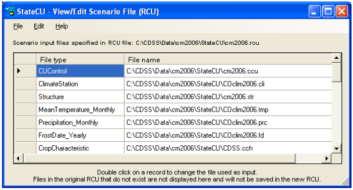
2.5.1 - Input File List
The Input File List command allows the user to view and edit individual input files listed in the response file of a scenario. When the Input File List command is selected from the Edit menu, the View/Edit Scenario File (RCU) window (Figure 20) is activated. The user can then double click on a file name, prompting an Open File window, in which the user can choose individual files located on any available disk drive or directory. Note that any input files listed in the original response file that do not exist are not listed in the View/Edit Scenario File (RCU) window and will not be saved in the new response file. The Copy option under the Edit menu allows the user to copy the input file names and paste the list in an external application, such as a text editor or spreadsheet. Utilize the Edit…Select All option or individually select or deselect input file names to copy by holding down the CTRL key while selecting file names with the LEFT mouse button.
Figure 20 - Input File List Window (see also the full-size image)
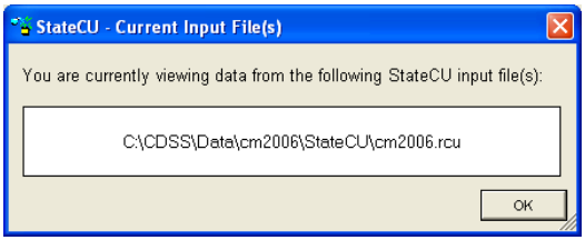
To save changes to the Input File List, select Save from the File menu. This command saves changes over the active response file. The Save As… command allows the response file to be saved in a different location or to a different name. The name of the active response file displayed in the View/Edit Scenario File (RCU) window can be determined by selecting the Input File Info command under the Help menu (Figure 21).
Figure 21 - Input File Information Window (see also the full-size image)
A File menu and Help menu similar to those shown above are provided for each command under the Edit menu.
2.5.2 - Model Control Options
The Model Control Options window displays the information and parameters that control a StateCU execution. With a Structure Scenario, the information is organized by three data groups which appear as ‘folder tabs’: General, Analysis Options, and More Options. The information available under each data group is viewed by clicking the folder tabs. Only the information shown under the General tab and a limited set of options under the Analysis Options tabs are provided for a Climate Station Scenario. The following should be noted when editing the model control parameters:
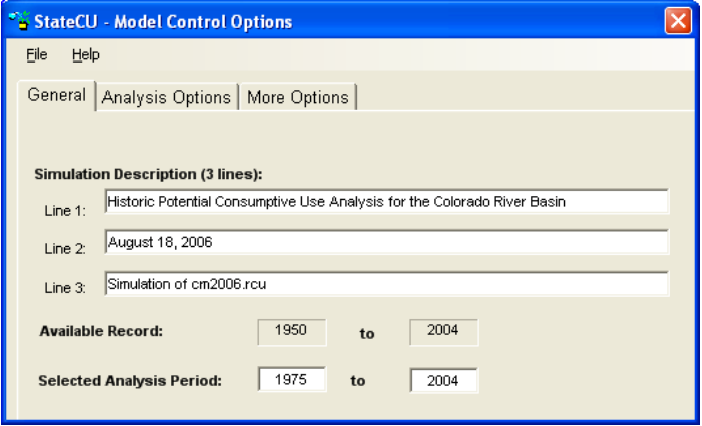
General (Figure 22):
- Simulation Description – Three lines are available to describe the simulation.
- Selected Analysis Period – Must be a subset of the Available Record (which is the first and last year of data that is available in every input file containing time series data).
Figure 22 - Model Control Options - General (see also the full-size image)
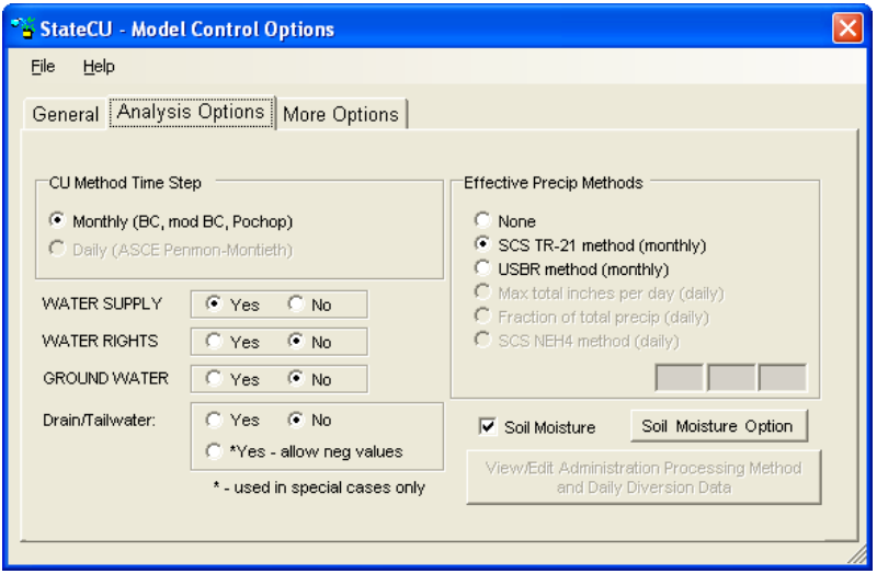
Analysis Options (Figure 23):
- CU Method Time Step – This option indicates whether the scenario uses a monthly consumptive use method (i.e. Original Blaney-Criddle, Modified Blaney-Criddle, or Pochop) or a daily method (i.e. ASCE Penman-Monteith). Daily climate data files must be included in the response file for the daily option to be activated.
- Effective Precipitation Methods – This option displays the effective precipitation methods that are available for the scenario. If the effective precipitation method is turned off (e.g. ‘None’), then StateCU estimates the total potential crop consumptive use. The effective precipitation methods available under a monthly consumptive use analysis include the SCS TR-21 method and the USBR method, as described in Section 3.1.2. Under a daily consumptive use analysis, the user can apply either a monthly or daily effective precipitation method. The daily effective precipitation methods include maximum effective inches per day, a fraction of the daily precipitation that is effective, or the SCS NEH4 method, as described in Section 3.1.6.
The following Analysis Options are only available under a Structure Scenario:
- Water Supply – This option should be selected to calculate water supply-limited crop consumptive use. Water supply information must be available for the Selected Analysis Period.
- Water Rights – This option should be selected to group consumptive use as senior or junior to a usersupplied administration number(s). This option is only available if the Water Supply option is selected and a direct diversion rights file (*.ddr) is included in the scenario. The administration processing method and numbers can be viewed and edited by selecting the View/Edit Administration Processing Method command button as described in Section 2.5.2.1.
- Ground Water – This option should be selected to consider ground water supply (not available if Water Rights option is selected).
- Soil Moisture – This option should be selected to consider water stored in the soil moisture zone as a water supply for serving crop consumptive use (only available if the Water Supply option is selected). Soil Moisture variables are described in Section 2.5.2.4.
- Drain/Tailwater – This option should be selected if the scenario includes a drain file (*.dra) that contains supplemental tailwater, drain flows or other off-river supplies not included in diversion records. If the drain file contains negative values, indicating non-irrigation diversions in the diversion file that need to be offset, select the ‘Yes – allow neg values’ drain option. See Section 4.28 for more information on drain file usage.
Figure 23 - Model Control Options - Analysis Options (see also the full-size image)
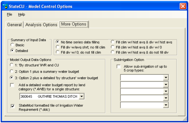
More Options (Figure 24):
- Summary of Input Data – This option allows a Basic or Detailed summary of all input used in the model (*.sum).
- Missing Data Fill Options – This option allows missing climate and diversion data to be filled ‘on-thefly’ to provide for a more complete consumptive use analysis. Utilizing one of these options allows
StateCU to fill missing climate and/or diversion data within the consumptive use simulation, however
does not replace missing data in the input file. The user can choose the following filling options:
- No time series data filling
- To fill missing diversion records based on average shortages and no filling of climate data
- To fill missing diversion records with zeros and no filling of climate data
- To fill both missing climate and diversion data with historic monthly averages
- To fill missing climate data with historic monthly averages and diversions with zeros
- To fill missing climate data with historic monthly averages and leave diversion data missing. Note that other options for filling missing climate and diversion data in input files are available through the TSTool DMI. Missing records can also be filled by editing or copying data through the GUI.
- Model Output Data Options – This option allows several levels of output data to be generated. Option 1 provides a matrix formatted crop irrigation water requirement summary (.cir) and water supply limited consumptive use summary (.wsl) when water supply is considered. Option 2 provides the output from Option 1 plus a summary water budget (.swb). Option 3 provides the output from Option 2 plus a detailed ‘by structure’ water budget (.dwb). In addition to the output generated by Options 1 through 3, the user can also choose to create a detailed water budget report by land category for a single structure (*.4wb), selected from a pull down list.
- StateMod Formatted file of Irrigation Water Requirement – This option creates an output file of irrigation water requirement (*.ddc) in the standard StateMod format.
Figure 24 - Model Control Options - More Options (see also the full-size image)
When the Save or Save As… command is selected from the File menu, the user will be prompted for a new control (.ccu) file name and the associated response file name. The new control file name will be written to the response (.rcu) file. Changes made under any of the tabs will be saved.
2.5.2.1 - View/Edit Administration Processing Method and Daily Diversion Data
The View/Edit Administration Processing Method and Daily Diversion Data command button on the Analysis Options tab in the Model Control Options window activates the Diversion/Administration Processing window (Figure 25). This window displays the information and parameters that control the determination of senior or junior diversions in a StateCU execution and the associated crop consumptive use characterized by priority (only available for a Structure Scenario).
Figure 25 - Diversions/Administration Processing Window (see also the full-size image)
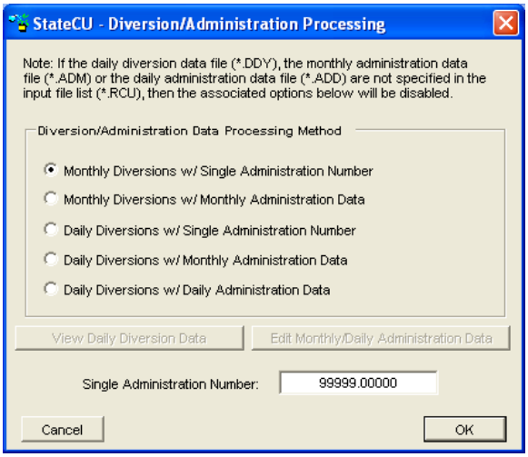
If water rights are being considered in the analysis (see Section 2.5.2), the user can select an option that will be used to ‘color’ the water supplies by user-defined administration number(s). The user can use daily or monthly diversion data, and apply daily, monthly, or a single administration number to those diversions. The available options are:
- Monthly diversion records and a single administration number.
- Monthly diversion records and monthly administration data.
- Daily diversion records and a single administration number.
- Daily diversion records and monthly administration data.
- Daily diversion records and daily administration data.
The first two options are available if a monthly historical direct diversion data file (*.ddh) is specified in the simulation input file list. The last three options are available if a daily water supply data file (*.ddy) is specified in the simulation input file list. User input monthly (second and fourth options) and daily (fifth option) administration numbers are stored in *.adm and *.add files, respectively, and are required to be on a calendar year basis. A single administration value (first and third options) is stored in the model control options file (*.ccu) with other model control parameters. See Section 2.5.1 for discussion on how to add these files to the simulation input list. See Section 4 for the format of these administration and diversion data files. If a daily diversion file is used to process water rights, daily diversions must add up to the total monthly diversions in the historical diversion data file (*.ddh).
To edit a single administration number, select either the first or third option and enter values in the Single Administration Number box. The user can view and edit diversion data and monthly or daily administration numbers (see Section 2.5).
To save changes to the processing method and, if option 1 or option 3 are selected, changes to the single administration number, select the OK command button and then select the Save or Save As… command from the File menu on the Model Control Parameters window. The save reloads the simulation input data files.
2.5.2.2 - View Daily Diversion Data Window
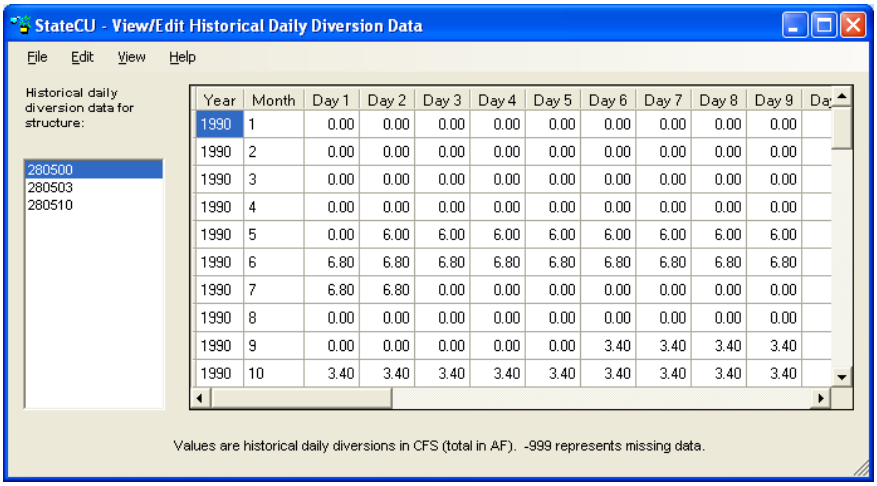
Selecting the View Daily Diversion Data command button on the Diversions/Administration Processing window activates the View/Edit Historical Daily Diversion Data window (Figure 26). This option is only available if a daily diversion file has been defined in the simulation input file list and a one of the daily diversion processing methods is selected on the Diversion/Administration Processing window. The user may select a structure to be viewed from the list of structures on the left side of the window; the diversion data will automatically refresh when a structure is selected. Daily diversion data can not be negative. Daily diversion data has units of cubic feet per second (cfs), with monthly totals in acre-feet.
The user has the ability to edit the diversion data through this window. See Section 2.5 for more information on how to edit data. To save changes to the daily diversion data for all structures, select the Save or Save As… command from the View/Edit Historical Daily Diversion Data…File menu.
Figure 26 - View Daily Diversion Data Window (see also the full-size image)
2.5.2.3 - Edit Monthly/Daily Administration Data
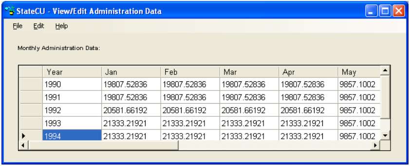
Selecting the Edit Monthly/Daily Administration Data command button on the Diversions/Administration Processing window activates the View/Edit Administration Data window (Figure 27). This option is only available if a monthly or daily administration file has been defined in the simulation input file list and one of the monthly or daily administration data processing methods is selected on the Diversion/Administration Processing window.
The user has the ability to edit the administration data through this window. See Section 2.5 for general information on how to edit data, however note that Scale and Add functions are disabled for this data type. Administration data must be a number between 0 and 99999. Changes to the administration data, select the Save or Save As… command from the View/Edit Historical Administration Data…File menu. The user will be prompted for a new monthly (*.adm) or daily (*.add) administration data file name and associated response file name. The administration data file name is written to the response (*.rcu) file.
Figure 27 - View/Edit Administration Data Window (see also the full-size image)
2.5.2.4 - View/Edit Soil Moisture Variables
The Soil Moisture Option button (only available for a Structure Scenario) on the Model Control Options window activates the Soil Moisture Variables window (Figure 28) which displays the information and parameters that control modeling of soil moisture in a StateCU execution.
Figure 28 - Soil Moisture Variables Window (with and without Water Rights) (see also the full-size image)
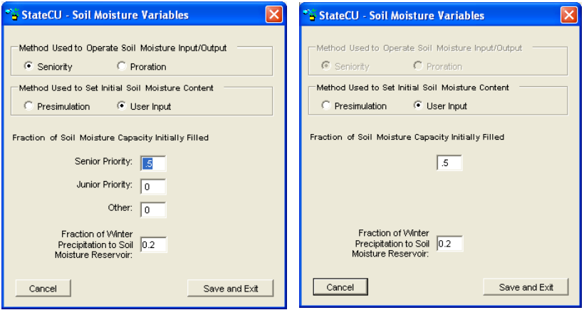
If the Water Rights option under the Model Control Options window is selected (see Section 2.5.2), the user can select an option in this window to operate the soil moisture reservoir on a ‘senior priority water first’ basis. If the Seniority option is selected, then any senior priority water available to the soil moisture reservoir is allowed to displace junior priority water existing in the reservoir. This option also allows the senior priority water in the soil moisture reservoir to be used (withdrawn) prior to the use of junior priority water. The effect of this Seniority option is to potentially increase the amount of consumptive use assigned to the senior priorities. If water rights are not being considered or the Seniority option is not selected, then the soil moisture reservoir will be operated on a ‘prorated’ basis. In Proration operation, soil moisture will be filled with the first available water and there will be no displacement of water already in storage. If considering water rights, soil moisture will be used under Proration operations based on the proportion of soil moisture in the various accounts. For example, if 10 acre-feet was withdrawn from a soil moisture reservoir where the senior priority soil moisture comprised 30 percent of the soil moisture and the junior priority soil moisture was 70 percent, then 3 acre-feet would be considered senior priority water and 7 acrefeet would be considered junior priority water.
The user can also select an option to allow initial soil moisture to be either set based on a Presimulation (of the same number of years as the true simulation) or by User Input values. The Presimulation mode starts out with soil moisture contents at zero and through a consumptive use simulation, allows the ending soil moisture values on a structure-by-structure basis to be assigned as the initial soil moisture values for the simulation. If User Input values are used, the user-defined percentages should add up to the percentage of total soil moisture estimated to be full at the start of the simulation. If considering water rights, the user is given an option of setting the percentages of the soil moisture capacity filled with Senior Priority (to the user-defined administration number) water, Junior Priority water, or Other (water not assigned to a priority). The user-defined values are applied in a consumptive use simulation to each structure being analyzed, regardless of that structure’s mix of junior and senior water rights.
The user can also choose to consider Winter Precipitation to Soil Moisture by entering the percentage of winter precipitation to be attributed to the soil moisture. The default is 20 percent, indicating a maximum of 20 percent of winter precipitation will be stored in soil moisture depending on available soil reservoir capacity. See Section 3.1.2.2 for details regarding the use of winter precipitation. To save changes, select the Save and Exit command button and then select the Save or Save As… command from the Model Control Parameters window. The save reloads the simulation input data files.
2.5.3 - Climate Station Information
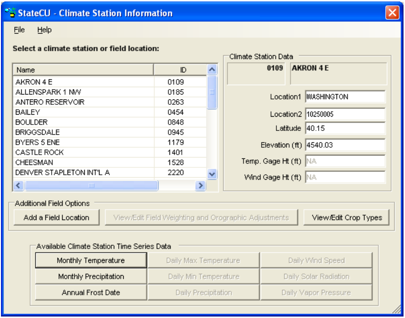
The Climate Station Information window allows the user to view and edit location information and climate data for a selected climate station. An example is shown in Figure 29 for a Climate Station Scenario. The Climate Station Information window is similar under both scenarios except for the following differences under a Structure Scenario:
- A field location can not be added. This option is only available under a Climate Station Scenario and allows the user to apply weighted climate station data and an orographic adjustment to climate station data (see Section 3.1.7).
- Climate station assignments and the crop types and acreages are associated with the actual structure and therefore viewed through the Structure Information window.
Each climate station is identified by its name, station ID, and a column indicating whether the climate station is included in the current scenario (see the Help…About Climate Stations menu for more information). To view and edit the climate station location information, select a climate station from the list and then view or edit the Location1 (e.g. county), Location2 (e.g. USGS Hydrologic Unit Code), Latitude, and Elevation data directly from the Climate Station Information window. With a daily consumptive use method, the Temperature Instrument Height and Wind Instrument Height can also be edited (entered in feet). If the user does not provide a temperature or wind instrument height, then the standard heights specified for the CoAgMet stations are used (4.92 feet = 1.5 meters for the temperature instrument and 6.56 feet = 2.0 meters for the wind instrument).
Changes made to any of the parameters under the Climate Station Data or Field Data entries must be saved before selecting a different climate station or field location from the list box. When the Save or Save As… command is selected from the File menu, the user will be prompted for a new climate station assignments (*.cli) file name and associated response file name. The climate station assignments file name is written to the response (*.rcu) file.
Figure 29 - Climate Station Information Window with a Climate Station (see also the full-size image)
2.5.3.1 - View/Edit Historical Climate Data
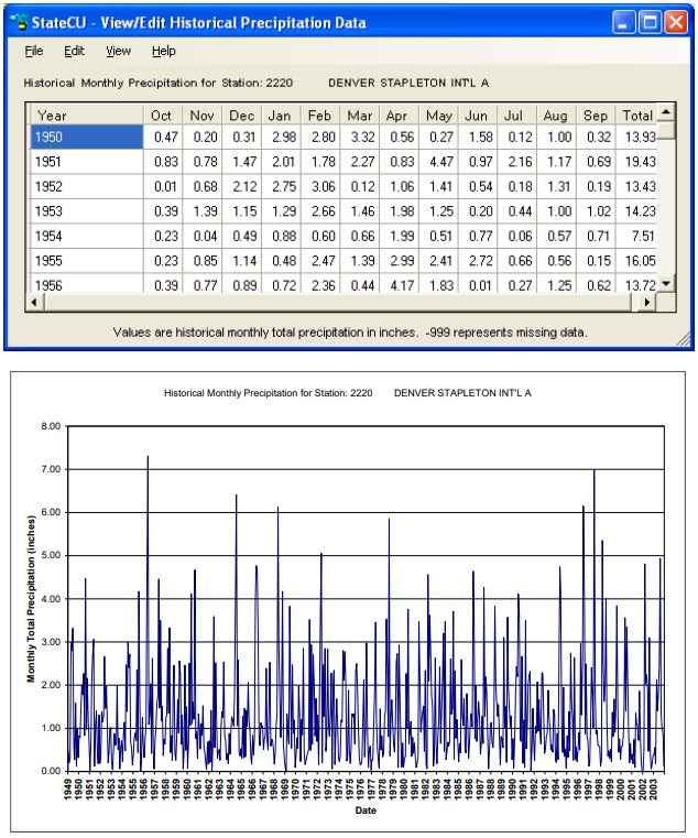
To view the monthly climate data, select a climate station from the list in the Climate Station Information window and then click on one of the data buttons under the Available Climate Station Time Series Data group. An example of the Monthly Precipitation window and results displayed from the View…Graph menu are provided in Figure 30. The other daily and monthly data windows are similar.
The user has the ability to edit the climate data through this window. See Section 3.5 for information on how to edit data through the GUI. When Save or Save As… is selected, the user will be prompted for a climate data file name (e.g. *.prc, *.tem) and associated response file name. The new crop distribution file name is written to the response (*.rcu) file.
Figure 30 - View/Edit Historical Climate Data (see also the full-size image)
2.5.3.2 - View/Edit Crop Types
With a Climate Station Scenario, the crop types are associated directly with the climate station (or field location if one has been added) and the analysis is performed on a unit acreage basis. With a Structure Scenario, the crop types are associated with the structure location and the analysis is performed for a specified total acreage and acreages of each crop type (See Section 2.5.4).
To view and edit the crop information, select a climate station from the list in the Climate Station Information window and then click the View/Edit Crop Types command button. The View/Edit Crop Acreage Data window provides the list of all available crop types in the crop characteristic (*.cch) file included in the scenario and the fraction of land associated with each crop type for each year of the analysis period in the upper portion of the window (Figure 31). The lower portion of the window sums the acreage percentages by year and can not be explicitly edited. Editing acreage percentages in the upper portion of the window will change the total acreage in the lower portion of the window. See Section 2.5 for general information on how to edit data through the GUI. Note that for a Climate Station Scenario, the sum of all crop percentages must equal 100 percent.
When Save or Save As… is selected, the user will be prompted for a new crop distribution (*.cds) file name and associated response file name. The new crop distribution file name is written to the response (*.rcu) file.
Figure 31 - Crop Information Window for a Climate Station Scenario (see also the full-size image)
2.5.3.3 - Field Location
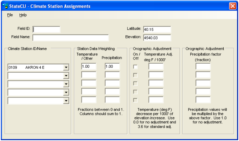
Climate station data typically represent climate data at the location of a climate station. With a Climate Station Scenario, a field location can be added and climate station data can be adjusted to the field location by specifying a latitude and elevation that are representative of the field location, assigning climate data from an individual climate station or weighting data from up to five different climate stations, and/or applying an orographic adjustment. Select the Add a Field Location from the Climate Station Information window to input a new field location in the Climate Station Assignment window (Figure 32).
- Field ID and Field Name – A unique Field ID and Field Name must be assigned by the user. Note that the Field ID can contain a combination of letters and numbers but no spaces. The Field ID can not be the same as a climate station ID included in the scenario.
- Latitude and Elevation – If latitude and elevation are not provided by the user, the program uses the latitude and elevations of the climate station(s) assigned (if more than one climate station is assigned, StateCU will calculate a latitude based on the temperature weights and the associated climate station latitudes).
- Climate Station ID/Name – If a climate station was highlighted when the Add a Field Location command button was selected, then the first climate station listed in the Climate Station Assignment window is the highlighted station. Climate stations can be added or changed by selecting from the dropdown list of available stations.
- Station Data Weighting – StateCU calculates the temperature and precipitation data for the field location using the data from each climate station assigned (up to five different stations), proportioned by the associated station weights (fractions), as described in Section 3.1.7. With a daily analysis, a weight (fraction) is specified for weighting the precipitation data and a temperature/other (fraction) is used to weight all of the other climate data. The GUI provides a warning but allows the user to continue if the weights for a given parameter (i.e. temperature data or precipitation data) do not each sum to 1.0.
- Orographic Adjustment – With a monthly consumptive use analysis method (Modified BlaneyCriddle, Original Blaney-Criddle, or Pochop), if elevations are provided for both the field location and the assigned climate station(s), then a temperature orographic adjustment can be used to adjust the monthly temperature data to the field location, as described in Section 3.1.7. This option is only available once a field elevation is provided, and must be turned on by selecting the On/Off option for the associated climate station(s). If the user chooses to apply an orographic adjustment to precipitation data, enter a factor that represents the average annual precipitation at the field location compared to the average annual precipitation at the climate station. This factor is applied to monthly precipitation data. When the orographic adjustment is initially turned ‘on’ through the StateCU GUI, the GUI displays the default temperature adjustment of 3.6 degrees Fahrenheit per 1,000 feet and the default precipitation adjustment of 1.0 (no adjustment). These default adjustments can be changed and saved through the GUI. An orographic adjustment is not currently allowed for the daily ASCE Standardized PenmanMonteith method.
Figure 32 - Climate Station Assignments Window (see also the full-size image)
When the Save or Save As… command is selected from the Climate Station Assignments window, the Crop Information window is activated allowing the user to input crop and acreage information to the new field location. Initially the GUI assigns the crop type for the new field location to the crop type associated with the first climate station assigned. The crop information can be edited in the Crop Information window as discussed in Section 3.5. When the Save or Save As… command is selected from the Crop Information window, the changes are made to the structure information (*.str) and crop distribution (*.cds) files and both files are written to the response (*.rcu) file.
Once a field location is created, it is added to the list of climate stations in the Climate Station Information window, and the climate stations and station data weighting can be viewed and edited by selecting the View/Edit Field Weighting and Orographic Adjustment command button from the Climate Station Information window. The associated crop distribution information can be viewed and edited by selecting the View/Edit Crop Types command button. The proportioned climate data can not be viewed directly – only the data associated with the climate stations used to create the field location can be viewed by selecting the original climate station(s) from the Climate Station Information window. Note that if the user does not provide a latitude for the field location (on the Climate Station Information window), the program will calculate a weighted latitude based on the latitude of the individual climate stations and the user-specified temperature weights.
2.5.4 - Structure Information
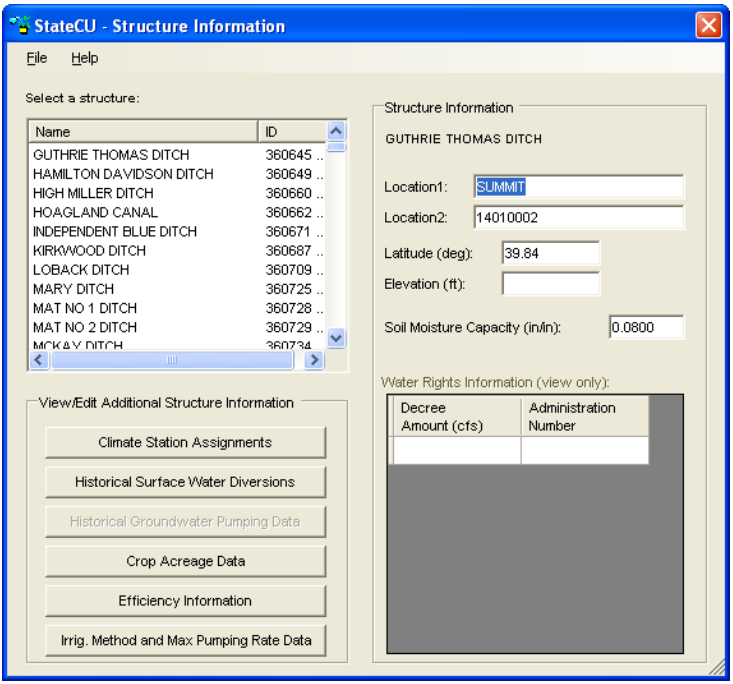
The Structure Information window (Figure 33) is only available for a Structure Scenario and allows the user to view and edit information from the input files required to define structure-specific parameters. These files include the structure location information (*.str) file, the parcel crop distribution (*.cds) file, the historic direct diversion (*.ddh) file, the water rights (*.ddr) file, the irrigation parameter yearly data (*.ipy) file, and the ground water pumping volume data (*.pvh) file. To revise information associated with a structure, select the structure from the structure list. The following should be noted when editing the structure information:
- Structure Information – The user can view and edit location identifiers (Location1, Location 2) typically representing County and USGS Hydrologic Unit Code respectively, in addition to latitude, elevation, and soil moisture capacity. If latitude is not provided, the program uses the latitude of the climate station(s) assigned. If soil moisture is not entered, no soil reservoir capacity will be estimated for the structure.
- Climate Station Assignments – Climate station assignments for a structure can be viewed and edited.
- Historical Surface Water Diversion – Historic surface water supply data for a structure can be viewed and edited. Missing data is indicated by a -999 value.
- Historical Ground Water Pumping Data – Historic ground water supply data for a structure can be viewed and edited. Missing data is indicated by a -999 value.
- Crop Acreage Data – Crop types and acreage for a structure can be viewed and edited.
- Efficiency Information – Conveyance and irrigation efficiency information for a structure can be viewed and edited.
- Irrig. Method and Max Pumping Rate Data – Irrigation method (flood or sprinkler), water source (surface water or ground water) information, ground water mode and monthly pumping limits for a structure can be viewed and edited.
- Water Rights Information – If a water rights analysis has been chosen, water rights associated with a structure can be viewed (non-editable) in the Water Rights Information box in the lower right corner of the Structure Information window.
Figure 33 - Structure Information Window (see also the full-size image)
When the Save or Save As… command is selected from the Structure Information window, only changes made to the location information are saved. The new structure location (*.str) file name is written to the response (*.rcu) file. Changes made to any of the other structure information related windows which are accessed from the Structure Information window must be saved directly under the associated windows.
2.5.4.1 - Climate Station Assignments
The Climate Station Assignments window is similar to the window used to add a field location under a Climate Station Scenario (Section 2.5.3.3 & Figure 32). It allows the user to view and modify the climate stations and weights assigned to each structure. With a monthly consumptive use analysis, StateCU calculates the temperature and precipitation data for a structure using the data from each selected climate station, proportioned by the associated weights (fractions). With a daily consumptive use analysis, StateCU calculates the maximum temperature, minimum temperature, wind speed, solar radiation, and vapor pressure for a structure using the data from each selected climate station, proportioned by the associated ‘Temperature/Other’ weights and the precipitation is calculated using the ‘Precipitation’ weights.
With a Structure Scenario and a monthly consumptive use analysis method (Modified Blaney-Criddle, Original Blaney-Criddle, or Pochop), the user has the option to adjust temperature and precipitation data through orographic adjustments. If elevations are provided for both the structure and the assigned climate station(s), then a temperature orographic adjustment can be used to adjust the monthly temperature data to a structure, as described in Section 3.1.7. Select On/Off options for each climate station under the Climate Station Assignments window for the selected structure to turn temperature and precipitation orographic adjustments on or off.
If the user chooses to apply an orographic adjustment to precipitation data, enter a factor that represents the average annual precipitation at the structure compared to the average annual precipitation at the climate station. This factor is applied to monthly precipitation data. When the orographic adjustments are initially turned ‘on’ through the StateCU GUI, the GUI displays the default temperature adjustment of 3.6 degrees Fahrenheit per 1,000 feet and the default precipitation adjustment of 1.0 (no adjustment). These default adjustments can be changed and saved through the GUI. An orographic adjustment is not currently allowed for the daily ASCE Standardized Penman-Monteith method.
When Save or Save As… are selected from this window, the user will be prompted for a new structure location (*.str) file name and the associated response file name. The new structure location file name will be written to the response (*.rcu) file.
2.5.4.2 - View Historical Surface Water Diversions
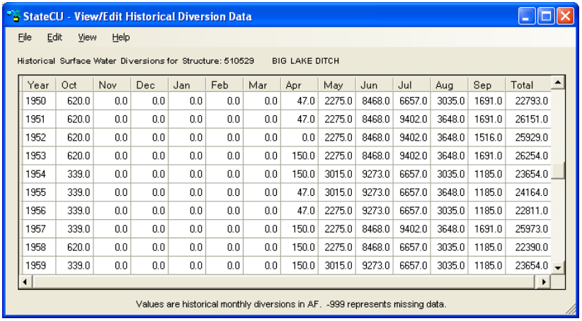
The View/Edit Historical Diversion Data window allows the user to view historic water supply data for the selected structure under the Structure Information window (Figure 34). Monthly surface water supply data is displayed for each year contained in the historical direct diversion (*.ddh) file. The user has the ability to edit the diversion data through this window. See Section 2.5 for general information on how to edit data through the GUI.
When Save or Save As… are selected from this window, the user will be prompted for a new historical direct diversion (*.ddh) file name and the associated response file name. The new historical direct diversion file name will be written to the response (*.rcu) file.
Figure 34 - View/Edit Historical Diversion Data Window (see also the full-size image)
2.5.4.3 - View Historical Ground Water Pumping Data
The View/Edit Historical Pumping Data window allows the user to view historic pumping data for the selected structure under the Structure Information window. Note that the user must select the Ground Water Analysis Option in the Model Control Options window to enable the Historical Ground Water Pumping Data button. Monthly pumping data is displayed for each structure contained in the ground water pumping file (*.pvh) file. Note that pumping data is not required for all structures listed in the structure file (*.str). The pumping data window is similar to the historical diversion data window, as shown in Figure 34, in both display and functionality. The user has the ability to edit, copy, paste, graph and save pumping data through the same methods as described in Section 2.5.
2.5.4.4 - View/Edit Crop Acreage Data
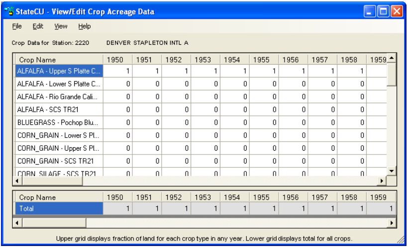
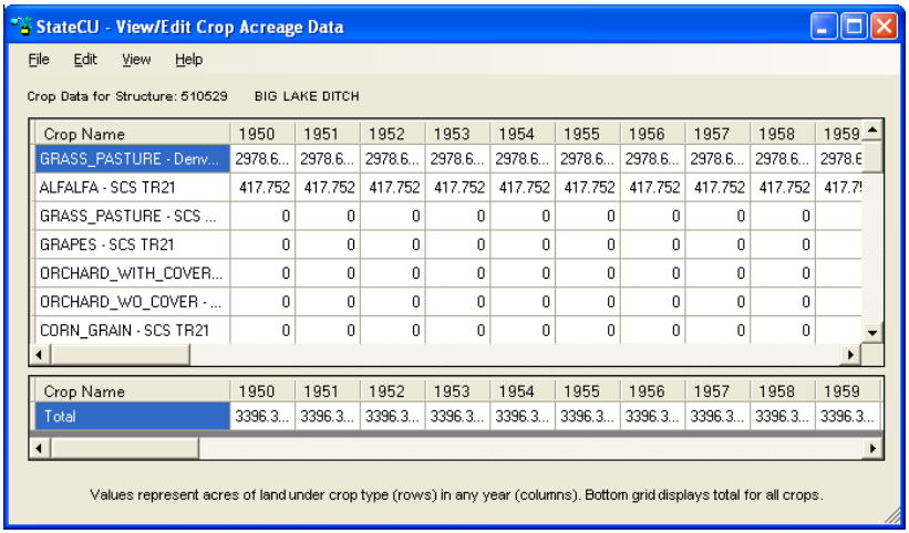
The View/Edit Crop Acreage Data window with a Structure Scenario is similar to the window used to view the crop types assigned to a climate station or field location with a Climate Station Scenario, except it reflects actual irrigated acreage, not percentages (Figure 35). With a Structure Scenario, the total acreage is specified and the portion of each crop type is specified as acres. For a given year, the GUI requires the sum of the acreage under each crop type to equal the total acreage. The View/Edit Crop Acreage Data window displays the crops for which there is acreage data at the top of the crop list in the upper portion of the window. The lower portion of the window sums the acreage by year and can not be explicitly edited. Editing acreage in the upper portion of the window will change the total acreage in the lower portion of the window. Note that only crops included in the crop characteristic and crop coefficient files are shown and can be assigned acreage. See Section 2.5 for general information on how to edit data through the GUI.
When the Save or Save As… command is selected from the Crop Information window, the changes will be made to the crop distribution (*.cds) file and the new file name will be written to the response (*.rcu) file.
Figure 35 - Crop Information Window with a Structure Scenario (see also the full-size image)
2.5.4.5 - View/Edit Historical Efficiency Data
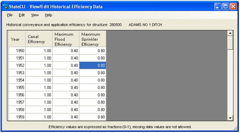
The Water Use Efficiencies window (Figure 36) allows the user to view and edit the annual conveyance and maximum irrigation efficiencies for the selected structure under the Structure Information window. Enter annual canal conveyance efficiency, maximum flood irrigation application efficiency and maximum sprinkler irrigation application efficiency parameters for each structure. The user has the ability to edit the efficiency data through this window. See Section 2.5 on general information on how to edit data through the GUI. Efficiency data must be input as a decimal (values 0 through 1 are allowable). Missing efficiency data (-999) is not allowed in the irrigation parameter yearly data file (*.ipy).
When Save or Save As… is selected, the user will be prompted for a new irrigation parameter yearly data (*.ipy) file name and associated response file name. The new irrigation parameter yearly file name will be written to the response (*.rcu) file.
Figure 36 - View/Edit Historical Efficiency Data Window (see also the full-size image)
2.5.4.6 - View/Edit Irrigation Method and Maximum Pumping Rate Data
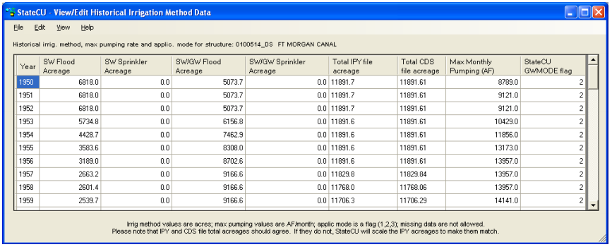
The View/Edit Historical Irrigation Method Data window (Figure 37) allows the user to view and edit annual acreage data associated with source and irrigation application method for the selected structure under the Structure Information window.
Acreages associated with surface water-only flood irrigation, surface water-only sprinkler irrigation, surface and ground water flood irrigation, and surface and ground water sprinkler irrigation are stored in the irrigation parameter yearly data (*.ipy) file. If land is only served by ground water, it should be assigned to the surface and ground water categories. The annual acreage data by crop type are stored in the crop distribution (*.cds) file. For a given year, the StateCU GUI requires the sum of the acreages in all four land use categories to equal the total irrigated acreage listed by crop type in the crop distribution (*.cds) file. For comparison, the GUI displays the total irrigated acreage from the crop distribution (*.cds) file next to the Total IPY file acreage column in this window. Any changes to the total irrigated acreage should first be made to the crop distribution file under the Crop Acreage Data window (Section 2.5.4.4). Once the revised total irrigated acreage by crop type is saved through the Crop Acreage Data window, the user can revise the acreage listed under the four land use categories in the View/Edit Historical Irrigation Method Data window. If the acreages listed in the irrigation parameter yearly file do not match the acreage stored in the crop distribution file, StateCU will scale the *.ipy acreages to match the *.cds acreages during the consumptive use analysis. The scaled data will not override the data stored in the irrigation parameter yearly file. After running StateCU, the log file will list the number of structures that were scaled to match. The maximum pumping rate and ground water mode can also be viewed and edited from this window. See Section 3.3 for information on ground water modes 1, 2 and 3. Note that data associated with ground water supply in the *.ipy file will only be considered in a structure scenario when the ground water supply option has been set in the Model Control Options window (see Section 2.5.2).
The user has the ability to edit the *.ipy acreage, pumping and ground water mode data through this window. See Section 2.5 for general information on how to edit data through the GUI. The user can not edit the Total CDS file acreage through this window; it is displayed as a comparison to the Total IPY file acreage data. No negative acreage data can be stored in the irrigation parameter yearly file.
When Save or Save As… is selected, the user will be prompted for a new irrigation parameter yearly data (*.ipy) file name and associated response file name. The new irrigation parameter yearly data file name will be written to the response (*.rcu) file.
Figure 37 - View/Edit Historical Irrigation Method Data (see also the full-size image)
2.5.5 - Crop Characteristics/Coefficients
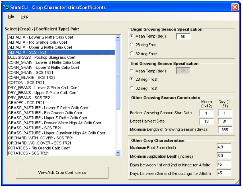
The Crop Characteristics/Coefficients window (Figure 38) displays information contained in the crop characteristics file (*.cch). The user can revise the criteria that set the beginning and ending of the growing season, other growing season constraints, maximum root zone depth, and maximum application depth for each crop and cutting parameters for alfalfa by selecting the crop from the crop list. The beginning and ending of the growing season specifications are compared to the other growing season constraints to determine the actual beginning and ending of growing season applied with the model. The latest date is used for the beginning of the growing season and the earliest date is used for the end of the growing season. For example, if the Earliest Growing Season Start Date is specified as May 15 and the Begin Growing Season Specification based on temperature results in a start date of April 28, the Earliest Growing Season Start Date is used.
Individual parameters for a selected crop type can be revised by using the radio controls and entering new information. Crop characteristics associated with a crop type that was not included in the loaded dataset can not be created through the GUI but rather must be added to the crop characteristic file through a text editor or StateDMI. When Save or Save As… is selected from this window, the user will be prompted for a new crop characteristic file name and the associated response file name. The new crop characteristic file name will be written to the response (*.rcu) file.
Figure 38 - Crop Characteristics/Coefficients Window (see also the full-size image)
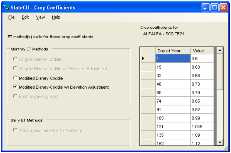
2.5.5.1 - View/Edit Crop Coefficients
The View/Edit Crop Coefficients command button activates the Crop Coefficients window (Figure 39)
which displays the crop coefficients for the selected crop type. Crop coefficients are developed for a
particular consumptive use method (e.g. Original Blaney-Criddle, Modified Blaney-Criddle, Pochop, or
ASCE Standardized Penman-Monteith) which is specified in the crop coefficient file. The StateCU GUI
displays the ‘valid’ consumptive use methods for a selected crop type and does not allow the user to switch
between methods except to add or take away the elevation adjustment within the Modified or Original
Blaney-Criddle methods. Note that the elevation adjustment is specified for a particular crop type, as
discussed in Section 3.1. If an elevation adjustment is specified for the ALFALFA.TR21 crop
coefficients, then the elevation adjustment is applied to the ALFALFA.TR21 portion of the scenario for any
climate station (under a Climate Station Scenario) or structure (under a Structure Scenario) with the crop
type of ALFALFA.TR21 specified. Crop coefficients associated with a crop type that was not included in
the loaded dataset can not be created through the GUI, but rather must be added to the crop coefficient file
through a text editor or StateDMI.
The user has the ability to edit the crop coefficient information through this window, however can not edit the Day of Year or the Percent of Season column. See Section 2.5 for general information on how to edit data through the GUI. Note that the Add and Scale functions are disabled for this data type.
When Save or Save As… is selected from this window, the user will be prompted for a new crop coefficient file name (*.kbc) and the associated response file name. The new crop coefficient file name will be written to the response (*.rcu) file.
Figure 39 - Crop Coefficients Window (see also the full-size image)