2.7 - Results Menu
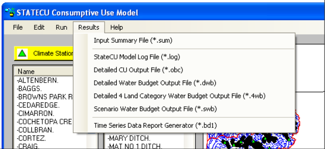
The Results menu options (Figure 40) allow the user to access the following output files:
- Input Summary File (*.sum)
- StateCU Model Log File (*.log)
- Detailed CU Output File (*.obc or *.opm)
- Detailed Water Budget Output File (*.dwb)
- Detailed 4 Land Category Water Budget Output File (*.4wb)
- Scenario Water Budget Output File (*.swb)
- Time Series Data Report Generator (*.bd1)
Note that the Detailed CU Output File has an extension of *.obc for the monthly consumptive use methods (Modified Blaney-Criddle, Original Blaney-Criddle, or Pochop) and an extension of *.opm for the daily ASCE Standardized Penman-Monteith method. The output files available under the Results menu depend on the settings under the More Options tab of the Model Control Options window (Section 2.5.2). The StateCU FORTRAN model generates all the output file options, with the exception of the Report Generator, and the GUI opens these output files using Microsoft Notepad. Section 5 discusses the each of these FORTRAN output options in detail. The Time Series Data Report Generator is discussed below in Section 2.7.1.
Figure 40 - Results Menu Commands (see also the full-size image)
2.7.1 - Time Series Data Report Generator
When the user runs a scenario, StateCU creates a binary file (*.bd1) with the results. The StateCU Time Series Data Tool (Figure 41) allows the user to view simulation results from this binary file in graphical, tabular, or summary formats. If the loaded scenario has been run, the Time Series Data Tool displays the binary file associated with the current scenario. The user can also search for an existing binary file through either selecting the Browse for File command button. Using this approach, results from multiple scenario runs can be compared.
Once a binary file is loaded, the user can view data associated with a climate station or structure by selecting the Add Row from Data Source command button. Once a row has been added, clicking on the ID (Name) field will provide the user with a list of available climate stations (for a Climate Station Scenario) or structures (for a Structure Scenario), or the user can select ‘All Structures’ stored in the binary file. The user must select one of the climate stations or structures in the list or other summary structure options to populate the ID (Name) field. Clicking on the Data Type field will provide the user with a list of available data for the current input dataset. Again, the user must click on one of the data types in the list to populate the Data Type field. The Begin Year and End Year can be selected to view a subset of the available period of record. Repeat the process discussed above to add as many rows as desired. The user can choose to save a created list of structures and data types by selecting the Save Current Record Set option under the File menu. The user can delete a series from the graph template by clicking on a row and selecting the Delete Selected Row command button or delete all rows by selecting the Delete All Rows command button. Select the Open Existing Record Set from the File menu to reload a previously created template.
The list of available data types is dependent upon the type of scenario, level of analysis and modeling options use to create the simulation binary file, as defined in the CU control file. Options may include: potential consumptive use, water supply limited consumptive use, surface water supply, ground water supply, consumptive use from direct diversions, consumptive use from ground water, consumptive use from soil reservoir, calculated surface water efficiencies, and calculated ground water efficiencies. Ground water output options are available only for scenarios that include ground water input data. Note that some output types and reports have restrictions on the number of structures or data types that can be included in the report or summary.
Note that under a daily analysis (e.g. ASCE Standardized Penman-Monteith), only the monthly totals can be viewed through the Time Series Data Tool. Daily results can be viewed from the *.opm output file.
Figure 41 - Time Series Data Tool (see also the full-size image)
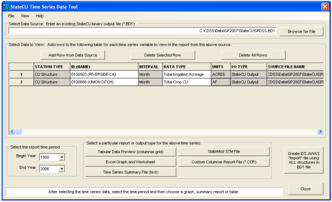
To create and view a graph, select the Excel Graph and Worksheet command button. The Tabular Data Preview, Time Series Summary File, and StateMod STM File command buttons can also be selected to view and save the data in tabular and summary formats used in the State’s other DMIs. The Custom Columnar Report File command is used to view and compare two or more columns of data generated for one structure. Select the Create IDS AWAS ‘Import’ File button to format the data from all structures stored in the binary file into AWAS import files for use in an IDS AWAS analysis. Data stored in a binary file can also be viewed through TSTool. To view the binary file in TSTool, open the TSTool application, select ‘StateCUB’ as the input type, and navigate to the *.bd1 file through the standard ‘Open File’ window. The available binary file parameters can then be accessed, modified and viewed through TSTool.
2.7.1.1 - Time Series Graph and Worksheet
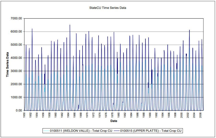
The StateCU GUI uses Excel to display graphical results (Figure 42) selected when the Time Series Graph (Excel) command button is selected from the Time Series Data Tool. The StateCU GUI opens Excel in a separate window and the time series data are provided under a worksheet labeled Data. Each row specified under the Time Series Data Tool is provided in a separate column of the Excel worksheet, and labeled with the ID (Name), Data Type, Units, and the binary file name and path. A single graph displaying all of the exported data is provided under a separate worksheet labeled Graph. Note that units may not be consistent. The StateCU GUI does not automatically save the results exported to Excel, however the Excel window will prompt the user for changes before closing. If Excel is not available on the user’s computer, the Time Series Graph option is not available.
Figure 42 - Time Series Data Tool Graphical Results (see also the full-size image)
2.7.1.2 - Tabular Data Preview
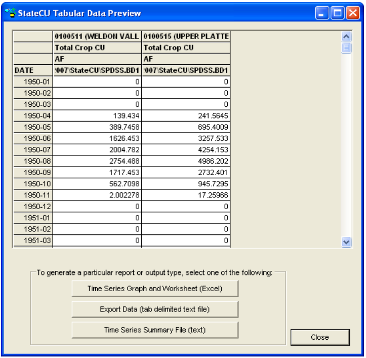
The StateCU GUI displays data in tabular format (Figure 43) when the Tabular Data Preview command button is selected from the Time Series Data Tool. The StateCU GUI opens a separate window displaying each row specified under the Time Series Data Tool in a separate column labeled with the ID (Name), Data Type, Units, and the binary file name and path. The tabular results can be saved to a tab-delimited text file by selecting the Export Data command button. View the tabular data using Excel by selecting the Time Series Graph and Worksheet button or view a text file of the data using Notepad by selecting the Times Series Summary File button, both located at the bottom of the Time Series Table window. Data can not be saved through the tabular preview window; however the data can be saved through each of the viewing and exporting options available at the bottom of the window. Select the Close button to return to the Time Series Data Tool window.
Figure 43 - Time Series Table (see also the full-size image)
2.7.1.3 - Time Series Summary
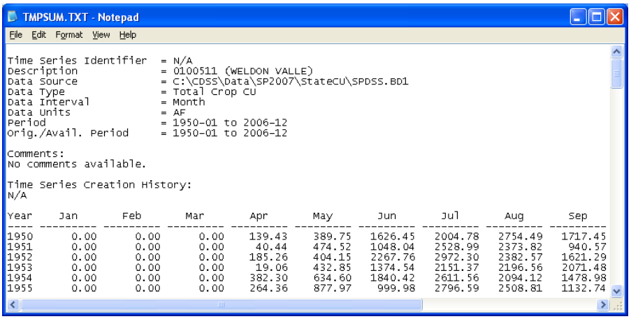
The StateCU GUI uses Microsoft Notepad to display summary results (Figure 44) when the Time Series Summary File button is selected from the Time Series Data Tool. The StateCU GUI opens Notepad in a separate window. Each row specified under the Time Series Data Tool is provided as a standard summary report within the file, similar to that used by the State’s other DMIs. The StateCU GUI does not automatically save the results exported to Notepad. To save results, the user must save the summary report from Notepad before closing the Notepad window.
Figure 44 - Time Series Summary File (see also the full-size image)
2.7.1.4 - StateMod STM File
Model results can be output as a StateMod formatted file (*.stm) by selecting the StateMod STM File button from the Time Series Data Tool. The StateMod STM File command is not used to display data, only to format and save data in a standard format used by the State’s other DMIs. The created *.stm file includes comments on StateCU report options used to generate the output, the name of the structure, data type, time period and file path name. A single StateMod output file can contain data from multiple CU Structures, however the same Data Type must be selected for each CU Structure (e.g. create one *.stm file containing irrigation water requirement data and a separate *.stm file containing total consumptive use). The *.stm file can be viewed through a text editor.
2.7.1.5 - Custom Columnar Report File
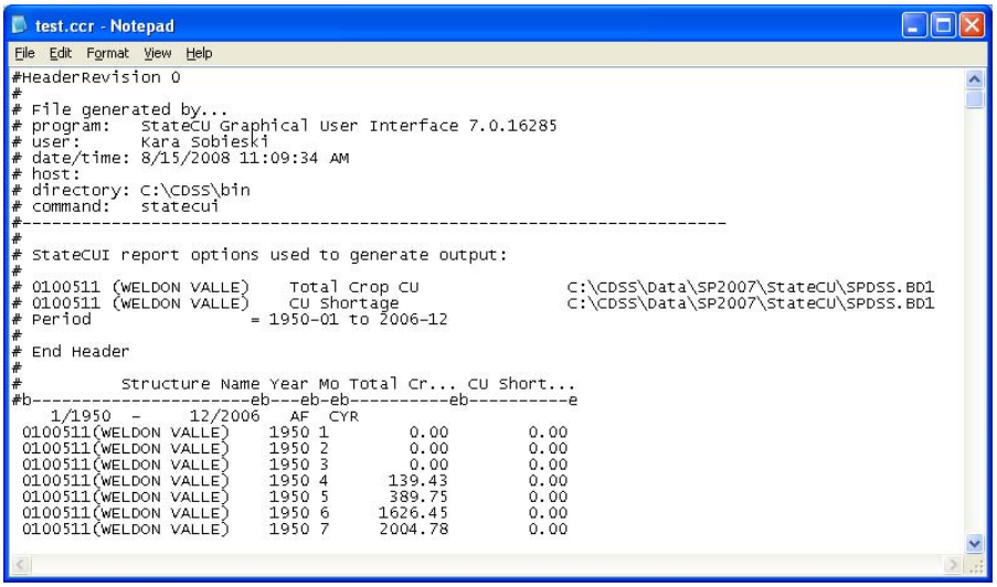
Simulation results for a single structure can be output to a custom column report (*.ccr) file by selecting the Custom Columnar Report File button from the Time Series Data Tool. This command is not used to display data, only to format and save data in a column format to compare multiple data types for a single structure. The created *.ccr file includes comments on StateCU report options used to generate the output, the name of the structure, data type(s), time period and file path name. The *.ccr file can be viewed through a text editor; an example *.ccr is shown in Figure 45.
Figure 45 - Custom Columnar Report File (see also the full-size image)
2.7.1.6 - IDS AWAS 'Import' File
The user can export monthly pumping and non-consumed applied water estimates from the Time Series Data Tool in a format that can be imported directly to the IDS Alluvial Water Accounting System (AWAS) program. IDS AWAS can then estimate the lagged stream depletions and accretions data based on userspecified aquifer parameters (e.g. Glover, SDF factors). The user can not specify which structures to include with this option; all structures available in the binary file will be included in the AWAS ‘Import’ file. For more information on the IDS AWAS program, see the Integrated Decision Support Group webpage at www.ids.colostate.edu. The IDS AWAS ‘Import’ file creation command is currently supported by version of IDS AWAS, Version 1.5.36. IDS personnel have indicated that future versions of IDS AWAS will continue to support this feature. Note that non-consumed applied water does not include water lost during conveyance to the farm.
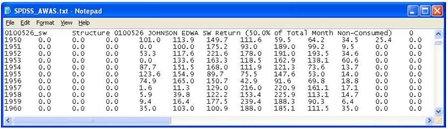
After loading the binary file, click on the Create IDS AWAS ‘Import’ File button. The GUI opens a window in which the user can rename the AWAS ‘Import’ file and indicate the directory to save the text file to. The GUI then opens a window asking the user to enter the percentage of unused water that is unlagged surface return flows (Figure 46). The default is zero percent; however the user can override the default with another percentage value then click OK. Note that the portion of unused water that is designated as unlagged surface return flows is assigned an SDF factor of zero, indicating immediate surface returns. Aquifer parameters can be edited in the AWAS program. The AWAS ‘Import’ file is then created and consists of three time series files; ground water pumping data, unlagged surface water return flow data, and lagged ground water return flow data. These time series are ready to be imported into the IDS AWAS program. An example of this file is shown in Figure 47. See Section 7.16 for more information on creating an AWAS ‘Import’ file.
Figure 46 - AWAS Import File - Surface Return Flow Percentage (see also the full-size image)
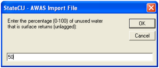
Figure 47 - AWAS Import File (see also the full-size image)